Option Pricing Models: How Are Options Priced?

Options are financial derivatives that give the holder (buyer) the right, but not the obligation, to buy (in the case of a call option) or sell (in the case of a put option) an underlying asset at a specified price (strike price) before or on a specified future date (expiration date).

Options are priced using various mathematical models, with the most widely used being the Black-Scholes model. This model, and others like it, take into account key market data and/or assumptions to determine the price of an option. 

The output of an options pricing model is typically viewed as a theoretical value. And this theoretical value may differ - at times significantly - from the current market price of an option.  

This may be due to a limitation of the pricing model, or due to a real-world factor in the options market, such as a disruption to supply/demand, an inefficient bid-ask spread, or some other factor. 

Such disruptions can develop during severe market corrections, or periods of significant uncertainty, but may also arise in other market environments, for a variety of reasons. Regardless, the output of an options pricing model - the theoretical value - often serves as a key reference point, and is typically used to evaluate (or compare against) the open market price of an option.

There are three common models used for pricing options: the Black-Scholes model, the Binomial Options Pricing Model (BOPM), and Monte Carlo Simulation. 

The Black-Scholes model offers a straightforward formula to estimate the prices of standardized options and is ideal for European-style options. The Binomial Model provides flexibility and is suitable for options that might be exercised early or for complex situations. Monte Carlo Simulation is a powerful numerical method used for handling complex options and non-standard market conditions.

The original Black-Scholes model was designed primarily to price European options, which are options that can only be exercised at expiration. American options, which can be exercised at any time before or on the expiration date, introduce additional complexity due to the possibility of early exercise. As a result, some financial engineers use the Binomial Model or other numerical methods when pricing American-style options. 

Different models exist because options can have varying characteristics, and market conditions can fluctuate. Moreover, a single model can’t necessarily capture all the nuances of option pricing across a wide range of scenarios and market environments. As a result, some market participants employ several different pricing models for specific types of options, situations, and/or market dynamics. In many cases, these models are proprietary, and not available to the public. 

The Black-Scholes model is a closed-form mathematical equation used to calculate the theoretical price of European-style options, which can only be exercised at expiration. 

This model provides explicit formulas for calculating the prices of both call and put options, incorporating factors such as the current asset price, strike price, time to expiration, volatility, and the risk-free interest rate. The Black-Scholes model is widely used for its simplicity and speed in pricing options with standardized characteristics.

The Black-Scholes formula, which can be used to calculate the value of a call option (C) or put option put (P), is shown below (for valuing a call option):

The primary inputs of the Black-Scholes formula include:

• Cumulative distribution function of the standard normal distribution (N)

• Current market price of the underlying asset (S)

• Strike price of the option (K)

• Time to maturity in years (T)

• Volatility of the underlying asset's returns (σ)

• Risk-free interest rate (r)

It should be noted that the Black-Scholes model encompasses not only the pricing formula (e.g. the equations shown above), but also the underlying assumptions and concepts that form the basis for option pricing. 

These assumptions include the efficient market hypothesis, constant volatility, continuous trading, and a risk-free interest rate. The model also introduces concepts like the log-normal distribution of asset prices and the concept of delta, gamma, theta, and vega as option Greeks.

The Binomial Options Pricing Model (BOPM) is another method used to estimate option prices, it arguably offers more versatility than the Black-Scholes model, but also requires more steps, calculations, and computational resources. 

The Binomial Options Pricing Model is a bit like a decision tree. Instead of assuming constant parameters, BOPM breaks down time into discrete intervals or steps, which allows one to theoretically model the underlying asset’s price movements at each step. By considering a range of possible price movements, and incorporating factors such as volatility and the risk-free interest rate, BOPM calculates the option's value at each step in the modeling process. 

This step-by-step modeling approach accommodates complex options, including American-style options (which possess early exercise features), making it a valuable tool for those market participants that seek a more sophisticated approach. The BOPM undoubtedly requires more computational resources, but it can be adapted to a wider range of market conditions, and therefore arguably delivers more accurate results. 

A Monte Carlo Simulation refers to a powerful options pricing approach that leverages randomness and statistical sampling to estimate option values. This methodology is akin to a “what if” analysis for options pricing. 

To conduct a Monte Carlo Simulation one must run thousands (or even millions) of simulations of potential future price paths for the underlying asset, each time considering various factors like volatility, interest rates, and dividends. These simulations create a wide range of possible scenarios, and for each scenario, the option's payoff at expiration is calculated. 

By averaging the payoffs across all simulations, the Monte Carlo Simulation provides an estimate of an option's expected value. 

This approach is particularly valuable for pricing complex options with non-standard features or in markets where the assumptions for some parameters may not be constant. When executed efficiently, the results of this approach can be highly accurate. However, Monte Carlo Simulations require extensive computational resources and software expertise, and are therefore typically conducted by financial engineers. 

Intrinsic value plays a crucial role in option pricing models, because it represents a fundamental component of an option's total value. The intrinsic value is the portion of an option's price that is based on the actual, or "in-the-money” (ITM), value of the option at a given point in time. 

Calculating intrinsic value is relatively straightforward - it represents the difference between the current market price of the underlying asset and the option's strike price. Additional details on intrinsic value are highlighted below. 

Call Options

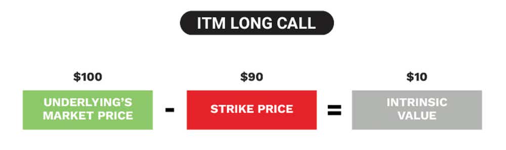
• For a call option, the intrinsic value is the positive difference between the current market price of the underlying asset (S) and the strike price (K) if S > K. In other words, it's the value that could be realized immediately by exercising the option and buying the underlying asset at the strike price.

• If S ≤ K, the call option has no intrinsic value, and it would not make sense to exercise the option, because you can buy the asset at a lower price in the open market.

Put Options

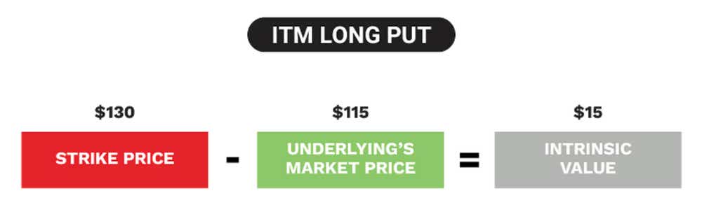
• For a put option, the intrinsic value is the positive difference between the strike price (K) and the current market price of the underlying asset (S) if K > S. It represents the value that could be obtained immediately by exercising the option and selling the underlying asset at the strike price.

• If K ≤ S, the put option has no intrinsic value because it would be more profitable to sell the asset at the open market price rather than exercising the option to sell it at the lower strike price.

In summary, intrinsic value is solely determined by the relationship between the current asset price and the option's strike price. It represents the real, tangible value that an option holds at a specific point in time based on these market conditions.

Extrinsic value, also known as time value, is another critical component within an option pricing model. It represents the portion of an option's price that exceeds its intrinsic value and is associated with the uncertainty and potential for future market movements. 

Extrinsic value quantifies the speculative or time-related value of the option beyond its current "in-the-money" or "out-of-the-money" status, and generally encompasses the following factors and assumptions:

• Time to Expiration (Theta): One of the primary drivers of extrinsic value is the time remaining until the option's expiration date. Extrinsic value tends to decrease as the expiration date approaches. The more time an option has until expiration, the greater the potential for market fluctuations that could make the option profitable, resulting in higher extrinsic value. Learn more about Theta.

• Implied Volatility (Vega): Changes in implied volatility, which measures market expectations for future price swings, impact extrinsic value significantly. Higher implied volatility typically leads to greater extrinsic value because there is a higher likelihood of substantial price movements, potentially benefiting option holders. Learn more about Vega.

• Interest Rates (Rho): The prevailing risk-free interest rate also affects extrinsic value. Higher interest rates can lead to increased extrinsic value, primarily for call options, as the opportunity cost of holding the option versus investing in risk-free assets rises.

• Dividends: For options on stocks, expected dividend payments can impact extrinsic value, particularly for put options. Changes to the dividend (raising or lowering) and/or the ex-dividend date can therefore trigger changes to an options value, which may or may not be significant in nature. 

In the options universe, the term “premium” is often used interchangeably to refer to the price that an investor or trader must pay to buy or sell an option. Premium and price both describe the amount of money associated with the option at a specific point in time. So, when you hear someone discussing the premium or price of an option, they are typically referring to the same concept – the monetary amount required to transact that option.

From that perspective, one can identify an option’s premium by looking at the options market, and checking the current price. 

However, to ascertain whether that market price is cheap, fair, or expensive, one would need to utilize an options pricing model, or base that evaluation on a metric like Implied Volatility Rank (aka IV Rank).

It should be noted that the real-world price of an option (e.g. the open market price) may differ from the theoretical value generated by an options pricing model. This may be due to a limitation of the pricing model, or due to a real-world factor in the options market, such as a disruption to supply/demand, an inefficient bid-ask spread, or some other factor. 

Such disruptions can develop during severe market corrections, or periods of significant uncertainty, but may also arise in other market environments, for a variety of reasons. 

Regardless, the output of an options pricing model - the theoretical value - often serves as a key reference point, and is typically used to evaluate (or compare against) the open market price of an option. 

Options pricing models are essential tools used by traders and investors to estimate the value (aka premium) of options. 

The most well-known options pricing model is the Black-Scholes model, which provides formulas to calculate the theoretical price of an option based on factors like the current asset price, strike price, time to expiration, volatility, and the risk-free interest rate. 

In addition to the Black-Scholes model, some market participants use the Binomial Options Pricing Model (BOPM), or Monte Carlo Simulations. However, both of these latter models require additional effort, mathematical skill, and computational resources. 

Different models exist because options can have varying characteristics, and market conditions can fluctuate. Moreover, a single model can’t necessarily capture all the nuances of option pricing across a wide range of scenarios and market environments. 

As a result, some market participants employ several different pricing models for specific types of options, situations, and/or market dynamics. In many cases, these models are proprietary, and not available to the public. 

It should be noted that the real-world price of an option (e.g. the open market price) may differ from the theoretical value generated by an options pricing model. This may be due to a limitation of the pricing model, or due to a real-world factor in the options market, such as a disruption to supply/demand, an inefficient bid-ask spread, or some other factor. 

Such disruptions can develop during severe market corrections, or periods of significant uncertainty, but may also arise in other market environments, for a variety of reasons. 

Regardless, the output of an options pricing model - the theoretical value - often serves as a key reference point, and is typically used to evaluate (or compare against) the open market price of an option.